Backpropagation Explained: How AI Models Actually Learn
At the heart of the AI revolution lies a remarkable process that allows machines to learn from their mistakes. This process, powered by concepts like Loss Functions, Epochs, and Backpropagation, is what transforms a “dumb” neural network into a powerful tool that can translate languages, identify images, or drive a car.
For anyone starting their journey in machine learning, these terms can seem intimidating. They are often surrounded by complex math and jargon. But the core concepts are surprisingly intuitive. In fact, a neural network learns in much the same way a human does: through trial, error, and gradual improvement.
This guide will demystify the training process. We’ll use a simple analogy—a basketball player learning to shoot free throws—to explain these three fundamental pillars of deep learning. By the end, you’ll have a clear, conceptual understanding of how AI models go from knowing nothing to making highly accurate predictions.
The Goal: Minimizing Error with a Loss Function
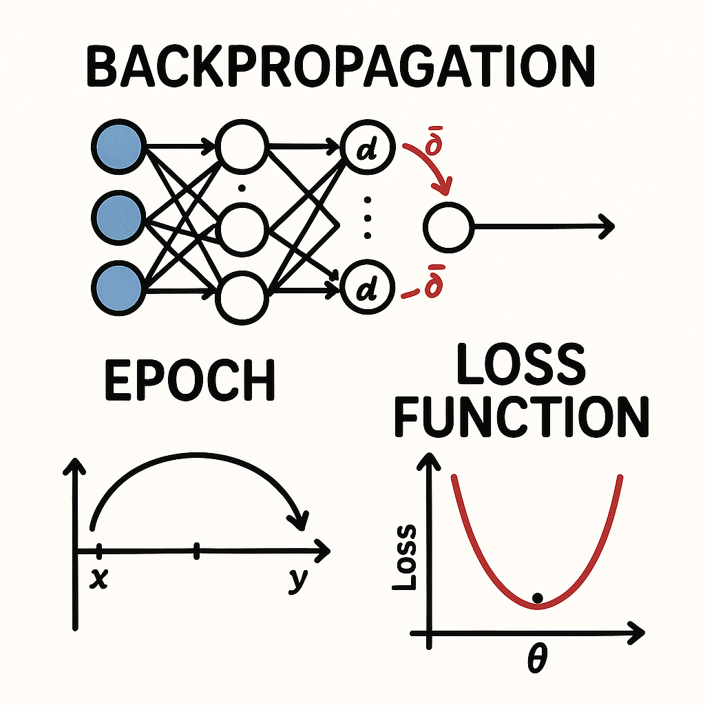
What is a Loss Function?
A Loss Function (also called a cost function or objective function) is a mathematical way of measuring how wrong a model’s prediction is compared to the actual, correct answer. It calculates a single number—the “loss” or “error”—that represents the penalty for a bad prediction. The higher the number, the worse the prediction was.
The entire goal of training a machine learning model is to find the set of internal parameters (weights) that minimizes the value of the loss function.
Analogy: Imagine a basketball player shooting a free throw. Their goal is to get the ball in the hoop (the correct answer). The player’s prediction is the actual shot. The loss function is the measurement of how far the ball was from the center of the hoop. A shot that misses entirely has a high loss. A shot that rattles in has a low loss. An “all-net” swish has a loss of zero.
There are many types of loss functions, each suited for different tasks. For example, “Mean Squared Error” is common for predicting numerical values (like a house price), while “Cross-Entropy Loss” is used for classification tasks (like identifying a cat vs. a dog). For a deeper technical dive, the documentation for libraries like PyTorch provides excellent explanations of each type.
The Process: Training in Epochs and Batches
What is an Epoch?
An epoch represents one full cycle where the machine learning model has seen and processed the entire training dataset. If a dataset is too large to fit into a computer’s memory at once, it’s broken down into smaller chunks called **batches**.
- Iteration: A single update of the model’s weights. This happens after processing one batch of data.
- Batch: A small subset of the total training data.
- Epoch: The completion of all batches, meaning the model has seen every single data instance one time.
Analogy: Our basketball player decides to practice by taking 1,000 free throws (the full dataset). They can’t do it all at once, so they decide to shoot in sets of 50 (the batch size). Each set of 50 shots is one batch. After they have completed all 20 batches (20 x 50 = 1,000), they have completed one epoch of practice. They will likely repeat this for many epochs to master their shot.
The number of epochs is a critical “hyperparameter” in model training. Too few epochs, and the model won’t have learned enough (underfitting). Too many, and it might memorize the training data too well and perform poorly on new data (overfitting). You can learn more about this in our guide to training and optimization.
The Engine: How Backpropagation Makes Learning Possible
What is Backpropagation?
Backpropagation (short for “backward propagation of errors”) is the core algorithm that allows a neural network to learn from its mistakes. After the model makes a prediction and the loss function calculates the error, backpropagation is the process that assigns blame for that error to every weight in the network. It then tells each weight exactly how to adjust itself—up or down—to reduce the error on the next attempt.
It does this using a mathematical technique called **gradient descent**, which finds the “slope” of the loss function and moves the weights in the opposite direction to find the lowest point of error. To dive deeper, Stanford’s renowned **CS231n course notes** offer a fantastic explanation.
Analogy: Our basketball player misses a shot to the left (a high loss). Backpropagation is the coach who analyzes the shot and says, “Your elbow was out by 5 degrees, and your wrist flick was 10 degrees too far to the right. On the next shot, tuck your elbow in slightly and adjust your wrist.” It doesn’t just say “you missed”; it provides specific, numerical feedback to every part of the shooting motion (every weight in the network) to guide the correction.
The Training Loop: Tying It All Together
So, how do these three concepts work together? In a continuous loop:
- The model takes a **batch** of data and makes a prediction.
- The **Loss Function** calculates the error between the prediction and the true labels.
- Backpropagation calculates the adjustments needed for every weight in the network.
- The model’s weights are updated.
- This process repeats for all batches until one **Epoch** is complete.
- The entire process is repeated for multiple epochs until the loss is minimized and the model is highly accurate.
This elegant loop of prediction, error calculation, and correction is what enables machines to learn, making it one of the most important concepts for any aspiring Machine Learning Engineer to master.
Frequently Asked Questions
Q: Is a bigger batch size always better?
A: Not necessarily. Larger batches can provide a more stable gradient and can be computationally efficient on GPUs, but they can sometimes cause the model to get stuck in a “local minimum” of the loss function. Smaller batches introduce more noise, which can sometimes help the model find a better overall solution. Finding the right batch size is a key part of model tuning.
Q: Why is it called “back”-propagation?
A: Because the error is calculated at the very end of the network (the output layer) and is then propagated backward, layer by layer, to the beginning of the network. The adjustments for the last layer are calculated first, then the second-to-last, and so on, all the way back to the input.
Q: Do I need to be an expert in calculus to use backpropagation?
A: No. Modern deep learning frameworks like PyTorch and TensorFlow handle all the complex calculus of backpropagation automatically. However, having a conceptual understanding of what it’s doing (finding the slope of the error to guide learning) is crucial for effective model building and troubleshooting.
Ready to Build Your Foundational Skills?
Understanding how models learn is a cornerstone of any serious AI learning path. Now that you’ve demystified the training process, you’re ready to explore more advanced concepts.
Explore Our Full Machine Learning Glossary


Leave a Reply